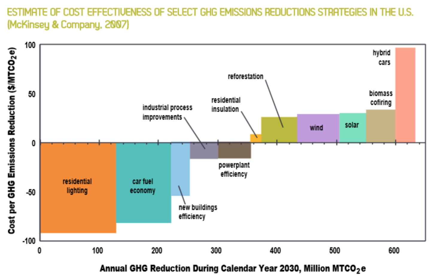
A Marginal Abatement Cost Curve (MAC curve or MACC) is a succinct and straightforward tool for presenting carbon emissions abatement options relative to a baseline (typically a business-as-usual pathway). A MAC curve permits an easy to read visualization of various mitigation options or measures organized by a single, understandable metric: economic cost of emissions abatement.

MAC curves are broken into discrete ‘blocks’. Each block represents an individual or set of similar carbon abatement measures. An example, based on the widely cited 2007 McKinsey & Company study and reproduced for the King County Strategic Climate Action Plan, is shown above combining various measures from different sectors. For each block (or measure), the width indicates the amount of potential carbon emissions abatement (tCO) while the height estimates the marginal cost of the carbon emissions abatement ($/tCO). Typically the blocks are ordered such that the lowest cost options, which may represent net cost savings (negative $/tCO, are shown first on the left with subsequent higher cost options proceeding to the right.
The first carbon-focused MAC curves date to the early 1990s, while similar curves for energy savings and other air pollutants first appeared in the early 1980s (Ekins et al.). The most well-known and widely used MAC curves have been compiled by McKinsey and Company starting in 2007 at the country level (Ekins et al
The usefulness of MAC curves
MAC curves are useful for framing carbon emissions abatement options, providing a tidy and accessible tool that orders measures on a simple economic metric ($/tCO). This allows measures from various sectors (e.g. transportation and power) to be compared on equivalent terms, serving as an initial lens of where abatement opportunities are potentially the largest and most cost effective. Therefore, MAC curves can be powerful for robust initial framing and identification of options to further evaluate. In this sense, MAC curves provide a great conversation starter from which deeper discussion and analysis can evolve with consideration of additional important dimensions and suitable policy options for unlocking the potential in each block.
The status of MAC curves for Washington state
To date, a Washington-specific MAC curve has not been developed, although there are examples at the national and state level that can provide some insight. A widely cited McKinsey & Company effort in 2007 gave a 2030 snapshot for the entire United States. However, this national perspective, aside from relying on many outdated assumptions, may not accurately portray more localized situations. As such an example, the 2015 King County SCAP highlights that “local energy sources are cleaner and result in fewer GHG emissions compared to national averages, energy efficiency strategies would likely be more costly per increment of GHG emissions reduction.”
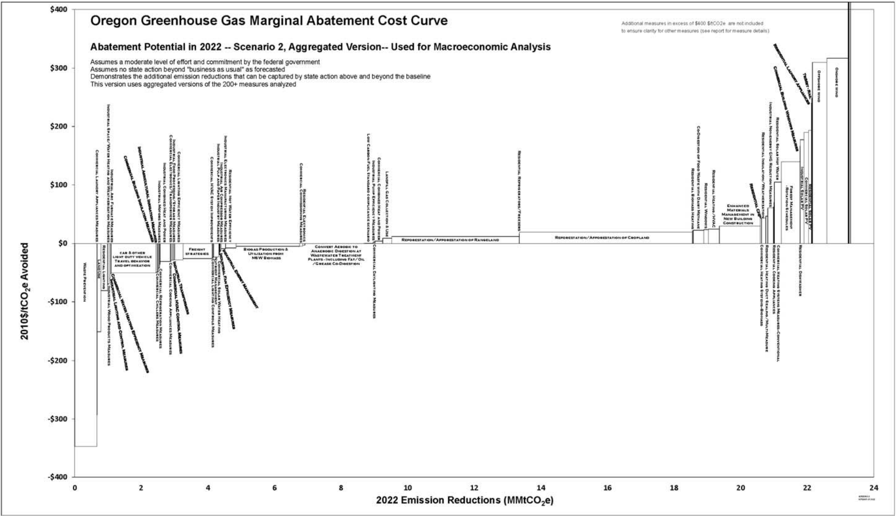
More recently and closer to home, Oregon funded a “McKinsey-like” cost curve carried out by the Center for Climate Strategies on an accelerated 3-month time frame. With the short time frame, this effort relied heavily on existing studies resulting in more of a ‘meta-analysis’ than comprehensive modeling effort. Despite the ‘meta-analysis’ nature and short project duration, the outputs are very comprehensive and well-documented, covering four sectors, three scenarios of effort and commitment and two ‘snapshot’ years (2022 and 2035). In part due to the short time-frame and in part inherent to MAC curves, the Oregon study gave overlapping reduction potential between measures only cursory treatment and views this as a big issue. The outputs show how complex a MAC curve can become as the number of sectors and types of measures under consideration expands:

Example of a MAC Curve for Oregon in 2022 (page 20).
Within Washington, there have been some pilot efforts and rumblings about developing MAC curves for the state. TheCERT Report to Governor Inslee described certain benefits of a MAC curve tool that is Washington-specific. These include gaining a better understanding of local emissions sources relative to California and Quebec in the case of a linked trading system, and “helping to identify least cost options for emissions reductions that should be pursued first and where technology enhancement efforts should be focused to keep total costs as low as possible.” One commenter, Steve Wright of the Chelan PUD, offered the following submission: “if we are going to seek out the most cost-effective means to reduce carbon emissions, we must have an analysis that provides a supply curve of potential carbon emissions compared against price.”
Some initial efforts that could feed into a Washington-specific MAC curve have surfaced, including a Pilot Cost Effectiveness Study with 13 actions (and evaluated along a third dimension: policy influence) as part of the 2015 King County Strategic Climate Action Plan and a 2013 report for CLEW by Leidos estimating $/tCOe for a subset of transport, energy conservation, and renewables options. At an institutional level, the UW Climate Action Plan includes a MAC Curve of it’s own.
ACKNOWLEDGING the limits of MAC curves
“The apparent simplicity and straightforwardness of the graphic MAC curve, with its summary and presentation of a great deal of complex numeric data in an easily-digestible form, often lead to these caveats being overlooked, so that excessive confidence is placed in the curves and the ranking of carbon abatement measures that they suggest” (Ekins, Kesicki, and Smith “Marginal Abatement Cost Curves: A Call for Caution”, UCL Energy Institute, April 2011).
If viewed as a useful springboard for more rigorous consideration of the various mitigation measures, including additional dimensions (e.g. development, health, barriers to implementation, how measures add up or relate to each other), MAC curves hold great promise.
Despite the appealing simplicity of a MAC curve, useful interpretation requires a great deal of care and expertise. Simply put, MAC curves alone are “not sufficient to base policy decisions on” (ERC Netherlands). If a MAC curve is recognized for what it contributes as “a device for creating like-for-like comparison around a limited range of considerations” it then “should not be the only tool used” (City Switch). To be useful, a MAC curve should “used with the understanding that it does not show how to abate, nor the economic impacts of abating” (MAPS Programme
Among the limitations of MAC curves highlighted in the literature are that the tool:
- Doesn’t capture non-market barriers to implementation, including indirect or non-transaction costs (ERC Netherlands Ekins et al.
- Contains very limited treatment of uncertainties in the underlying analysis and assumptions (e.g. technology economics, learning rates, choice of discount rates, time of retirement for working capital goods) (ERC Netherlands MAPS Technical Paper Ekins et al.
- Has difficulty capturing interactions between different measures that may limit the total abatement potential (City Switch Drumheller 2013). “Abatement measures interact, creating synergies and conflicts that mean that the cumulative outcome of two measures may be more than the sum of its parts, or less” (Ekins et al.
- Does not address dimensions other than direct costs, including strategic, operational, or political factors (City Switch). These may include both ancillary benefits (air and water pollution) or market failures (MAPS Technical Paper Ekins et al.). “In general, the MAC curve is unable to capture the wider social implications related to climate change mitigation” (Ekins et al.
In order for a MAC curve to be as robust and insightful tool as possible, care should be taken in the approach and interpretation of MAC curves. Ekins et al. suggest several recommendations for “the use of MAC curves by policy makers and others…to enable them to realize their potential in decision support”:
- Embrace complexity (“the usefulness of simple summary presentations of complex issues is limited”);
- Pay attention to the underlying assumptions (“keeping the assumptions and the MAC curve together can help ensure transparency, comprehensibility and accountability”);
- Always look beyond the estimated technology cost (“Basing decisions on estimated technology costs alone may not only fail to produce the promised carbon savings but also result in unintended or perverse consequences”);
- Understand path dependencies (“Abatement strategies are better presented and considered as scenarios or trajectories, in which decisions in one period influence the trajectory thereafter. Cumulative emissions are a more scientifically robust indicator of global warming commitment than abatement potentials in one or two horizon years.”)
If these caveats are treated appropriately, there is no doubt that a Washington-specific MAC curve could provide a great boost in catalyzing cost-effective strategies for meeting (or perhaps exceeding!) statewide greenhouse gas emissions standards (1990 levels by 2020, a further 25% reduction by 2035, and a 50% reduction relative to 1990 by 2050) and serve as a powerful tool for Washington businesses, utilities, and policymakers.
